In several occasions I needed to generate synthetic data with a desired level of spatial autocorrelation. Here I will show how to generate as many such fields as we need by using R, an open-source port of the S language for statical analysis. I will concentrate on two alternative ways of generating spatially correlated random fields (commonly known as unconditional Gaussian simulation), using the libraries gstat and fields.
1. Unconditional Gaussian simulation using gstat
Spatial modellers commonly use the term unconditional Gaussian simulation to refer to the process of generating spatially correlated random fields. For comparison purposes, the Figure 0 shows an example of a random field with no spatial correlation. The value of the measured property at one given cell is completely independent of the values of that property at neighbouring cells. This situation is very seldom (or I perhaps should better say never) found in nature, since spatially distributed variables always have a certain level of autocorrelation, i.e. co-variance between neighbours. This is often mentioned as the ‘geographical law’, stating that closer locations tend to have similar properties.
Generating spatially correlated random fields is interesting because it makes it possible testing different issues related to the statistical analysis of spatial data.
1.1. Generating the spatial field
We are going to use the gstat library, so we start by loading it:
library(gstat)
We create a 100 x 100 grid, and we convert it into a data frame (xyz structure) by taking all possible combinations of the x and y coordinates:
xy <- expand.grid(1:100, 1:100)
We give names to the variables:
names(xy) <- c('x','y')
Defining the spatial model and performing the simulations.
Second, we define the spatial model as a gstat object:
g.dummy <- gstat(formula=z~1, locations=~x+y, dummy=T, beta=1, model=vgm(psill=0.025, range=5, model='Exp'), nmax=20)
where formula defines the dependent variable (z) as a linear model of independent variables. For ordinary and simple kriging we can use the formula z~1; for simple kriging it is necessary to define a beta parameter too (see below); for universal kriging, if z is linearly dependent on x and y use the formula z~x+y. We are using simple kriging here. locations define the data coordinates, e.g. ~x+y in our case here. dummy is a logical value, and it needs to be TRUE for unconditional simulation. beta is used only for simple kriging, and is a vector with the trend coefficients (including an intercept); if no independent variables are defined the model only contains an intercept, i.e. the simple kriging mean. model defines the variogram model, as defined by a call to vgm. vgm allows defining the (partial) sill, range and nugget paramaters, as well as the variogram model type (e.g. exponential, gaussian, spherical, etc). Anisotropy can also be used. nmax defines the number of nearest observations that should be used for a kriging prediction or simulation.
Now we are ready to make as many simulations as we like based on the gstat object (four simulations in this example):
yy <- predict(g.dummy, newdata=xy, nsim=4)
1.2. Displaying the simulations
To see one realisation of the simulations:
gridded(yy) = ~x+y
spplot(obj=yy[1])

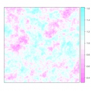
Figure 1. A spatially correlated random spatial field with mean=1, sill=0.025, range=5, exponential variogram model.
spplot, from the library sp, provides lattice (trellis) plot methods for spatial data with attributes. It’s only compulsory parameter is obj, which must point to an object of class Spatial; gstat objects belong to this class, so there’s no need to do anything extra. It is possible to show all four simulations in a single trellis plot:
spplot(yy)
1.3. Complete code
I include the complete code for convenience:
# unconditional simulations on a 100 x 100 grid using gstat
library(gstat)

# create structure
xy <- expand.grid(1:100, 1:100)
names(xy) <- c("x","y")

# define the gstat object (spatial model)
g.dummy <- gstat(formula=z~1, locations=~x+y, dummy=T, beta=1, model=vgm(psill=0.025,model="Exp",range=5), nmax=20)

# make four simulations based on the stat object
yy <- predict(g.dummy, newdata=xy, nsim=4)

# show one realization
gridded(yy) = ~x+y
spplot(yy[1])

# show all four simulations:
spplot(yy)
1.4. Variations
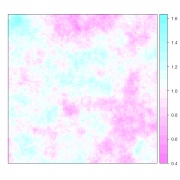
By modifying the range parameter in the variogram model it is possible to control the degree of spatial correlation. For example, by setting it at 15 instead of 5 we get a random field with a ‘coarser’ autocorrelation (Figure 2).
g.dummy <- gstat(formula=z~1, locations=~x+y, dummy=T, beta=1, model=vgm(psill=0.025, range=15, model='Exp'), nmax=20)

Figure 2. A spatially correlated random spatial field with mean=1, sill=0.025, range=15, exponential variogram model.
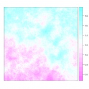
For including a linear trend surface in the simulation we can perform a universal kriging. For doing so it is necessary to specify it in the formula parameter as ~1+x+y, and coefficients for the x and y components need to be specified in the beta parameter. For example, the following defines a model with a spatial trend in the y dimension (Figure 3):
g.dummy <- gstat(formula=z~1+y, locations=~y, dummy=T, beta=c(1,0,0.005), model=vgm(psill=0.025, range=15, model='Exp'), nmax=20)

Figure 3. A spatially correlated random spatial field with mean=1, sill=0.025, range=15, y_trend=0.005, exponential variogram model.
The following code defines a model with a trend in both dimensions:
g.dummy <- gstat(formula=z~1+x+y, locations=~x+y, dummy=T, beta=c(1,0.01,0.005), model=vgm(psill=0.025, range=15, model='Exp'), nmax=20)
2. Unconditional Gaussian simulation using fields
Spatially correlated random fields can also be generated using the fields library. I put an example code here, and leave the details to the reader to investigate.
library(fields)
# load Maunga Whau volcano (Mt Eden) elevation dataset (matrix format)
data(volcano)

# reduce size
volcano2 <- volcano[10:55, 14:51]
filled.contour(volcano2, color.palette=terrain.colors, asp=1)
cols <- length(volcano2[1,])
rows <- length(volcano2[,1])

# create dataframe (xyz format)
X <- rep(1:cols, each=rows)
Y <- rep(1:rows, cols)
Z <- as.vector(volcano2)
volcano.df <- data.frame(X,Y,Z,cellid=1:cols*rows)
attach(volcano.df)
quilt.plot(Y,X,Z,nrow=rows,ncol=cols,add=F)

# create a spatial autocorrelation signature
# coordinate list
coords <- data.frame(X,Y)
# distance matrix
dist <- as.matrix(dist(coords))

# create a correlation structure (exponential)
str <- -0.1 # strength of autocorrelation, inv. proportional to str
omega1 <- exp(str*dist)

# calculate correlation weights, and invert weights matrix
weights <- chol(solve(omega1))
weights_inv <- solve(weights)

# create an autocorrelated random field
set.seed(1011)
error <- weights_inv %*% rnorm(dim(dist)[1])
quilt.plot(Y,X,error,nrow=rows,ncol=cols,add=F)

# create a variable as a linear function of the elevation
a <- 10
b <- 0.5
Z2 <- a + b*Z
quilt.plot(Y,X,Z2,nrow=rows,ncol=cols,add=F)

# add the autocorrelated error to the new variable
Z3 <- Z2 + error
quilt.plot(Y,X,Z3,nrow=rows,ncol=cols,add=F)

# export data (xyz format)
write.table(data.frame(X,Y,Z,Z2,Z3), file="data.txt", row.names=F, sep="\t")

Thank you for this clear explanation for how you generate random fields.
Thank you very interesing post, by the way do you know how to make lognormal random fields simulation?
Sequential Gaussian simulation would yield a normally distributed data at each point, i.e. with mean and standard deviation equal to the kriged mean and standard deviation. I am not sure about how to generate lognormal fields, but it is an interesting question and I will do a little research.
Que pequeño es el mundo! Buscando como simular procesos gaussianos en R y aquí te encuentro. Muchas gracias por las instrucciones!
Hi, I am working on simulating a gaussian random field and I want to incorporate a y trend (as in your example). I want this trend to be the same as in some data I have (higher values for larger y) — am I correct in thinking that you find the values for beta by looking at the coefficients of the linear model data~x+y? Doing this gives me beta=(0.73,0,-1.2) but I then get the trend in the wrong direction (higher values for smaller y). Where am I going wrong here?
Hi Laura, it’s difficult to say with so little information. The procedure you describe is basically right: you fit a linear model and look at the beta coefficients from that regression. I do not know why you get a negative beta for y, you should at your data and try to figure out…
Hi, this gives one a good starting point. in geoR, how would one differentiate a regular lattice from a fine grid?
Hi Mike, I don’t use geoR, I’m sorry.
Hi Sbegueria;
I’m new to this field, and hoping you can clarify some issues– although you don’t explicitly indicate this, but should I assume that GSTAT and FIELDS use ‘direct sequential simulation’ (a new concept for me) versus synthesizing a covariance matrix COV (and then using Cholesky, etc.)? If so, is one limited to generating a grid only with GSTAT, whereas for a COV matrix, any point distribution can work, but at the computational cost of Cholesky?
thanks!
Hi, the package produces simulation unconditional but i have the concern that algorithm used to simulation of those realizations.
Hi,
Thanks for this interesting post.Is that possible to generate spatially correlated multivariate random filed using gstat or any other package?
Hi Nish, although I’ve never tried it, in principle it should be possible via co-kriging. Please, let us know if you succeded.
Hi Santiago,
Excellent post.
I am using synthetic datasets in my doctoral research and I would appreciate if you could point me to papers where you (or others) have used the approach in this post to generate random fields.
Much appreciated
Sebastian
Sure, this is one example: Beguería S., Pueyo Y. (2009) A comparison of simultaneous autoregressive, generalized least squares models for dealing with spatial autocorrelation. Global Ecology and Biogeography 18, 273–279. — See more at: http://santiago.begueria.es/publications‑4/#sthash.TwPR0NaM.dpuf.
Also, but under review: Bias in the variance of gridded datasets leads to misleading conclusions about changes in climate variability.
Hi Santiago,
First of all, thank you so much for your reply. I don’t want to abuse your kindness but in your 2009 paper (the one you cited above) I can’t find any reference to generating synthetic spatially autocorrelated data with the method you show in this blog. Furthermore, the data mentioned is from Kissling & Carl (2008), which comes from the volcano dataset. There are also 2 datasets mentioned in which the spatial structure was degraded by sample reduction and coarsening.
Seems that I am missing something on how you used “gstat” or “fields” in generating synthetic data.
Please advice.
Thank you in advance.
Hi Sebastian, you’re totally right. We used the dataset of Kissling and Carl on our 2009 paper. Well, I know I used this method for some application when I wrote the post, but I don’t remember to have used it in any paper. There is one in press right now, but nothing you can refer to in your thesis, I’m sorry for that. Hopefully in some weeks there’ll be one example, when this paper will appear online.
Thank you for your reply Santiago. Looking forward to your upcoming paper!
Would you know of code to do the reverse; if you have a general matrix, extract the spatial auto-correlation function?
In the case of spatial data, I’m most familiar with using the functions
variogramandfit.variogramin thegstatpackage. You may want to have a look at the tutorial at https://cran.r‑project.org/web/packages/gstat/vignettes/gstat.pdf.Hi
I need to cross validate after simulation, how can I do that?
I used grf in package geor to simulate, I can cross validate its output but grf can’t simulate the exact formula like z#1 or z#x and so on unlike your commands.
So how can I cross validate your command?
My English isn’t good unfortunately.
Thanks in advance
Thank you very much~It’s great!
Thank you for this post. It’s very useful. I’ve still one question — how do you generate the first figure (with zero spatial correlation)?
Hi jn, as JoshO also noted there is an error in the first figure (it obviously has spatial correlation in it), I have corrected this in the post.
Thanks for this nice post. There are a few +/- important errors that you might want to fix (if that’s possible in a blog post): (1) Figure 0 does not, as claimed in the text “show[] an example of a random field with no spatial correlation.”; (2) The code block following the phrase “For example, the following defines a model with a spatial trend in the y dimension (Figure 3)” does not do what it claims. It sets formula=z~1+x+y, when it should be formula=z~1+y.
Hi JoshO. You’re right, I corrected both issues in the post, thanks a lot.
[…] These steps are repeated until all observations are given a value (Bivand et al., 2013). Note that another interesting post tackles the simulation of these gaussian random fields in […]
[…] ce que toutes les observations reçoivent une valeur (Bivand et al., 2013). A noter cet autre post qui s’intéresse de près à la simulation de champs gaussians aléatoires sur R (et qui a bien […]
I’m not sure that I understood your question. You can incorporate the variogram parameters that match your data directly into the function.
thank you for the post. but what if i have the correlation matrix already and i want to insert it as a given with the mean and cov?
I am trying to create a 10 x 10 matrix comprised only of whole numbers ranging from 1–10, with each integer represented 10 times (e.g., 10 1’s and 10 2’s), and a spatial correlation strength of 0.15. I’ve tried altering your code in both the ‘gstat’ and ‘fields’ packages, but cannot quite get the process to work. The closest that I have come is to constrain the matrix to numbers ranging from 1–10, but the output winds up including numbers with decimals. Do you have any suggestions? Thanks!
Hi Nathan. A fast solution could be to just round the values of your resulting field to have zero decimals with function
roundin R. Getting exactly 10 repetitions of each value between 1 and 10 is going to be much more difficult, and I’m not aware of any method to get that. Only approach that comes to mind is to repeat a number of simulated fields and reject all those that do not meet the criteria. There is a pretty efficient way to get a number of simulations with parameternsimof gstat’spredictmethod).Hi, thanks for this post! I have one question as I am completely new to this. I am generating landscapes with various levels of spatial autocorrelation, however, the “landscape” is already composed of cells varying from 0-.50. Is there any way to do exactly as what you explained, but with a raster that has predefined values? In your figures above, I see that the cells have a range of values of about .4 to 1.6.
Hi Stephanie. The parameter
betaspecifies the mean of your Gaussian field. In my example I set it to 1, and that’s why the data vary around that value. You can also control the standard deviation / variance of the field with the semivariogram parameters (psilland, if you want to use it,nugget).Thanks a lot! This is exactly what I needed.
[…] until all observations are given a value (Bivand et al., 2013). Note that another interesting post tackles the simulation of these gaussian random fields in […]