End of the story (this continues the previous post). I read one year of data for one HRU from the output.hru in R (), and I applied the water balance equation described in the linked posts. This is basically the following:
t <- 2:12
tt <- t-1
DStorage <- c(NA, SNOFALL[t] - SNOMELT[t] +
	SW_END[t] - SW_END[tt] + SA_ST[t] -
	SA_ST[tt] + DA_ST[t] - DA_ST[tt])
Flows <- PRECIP + IRR + GW_RCHG -
	ET - REVAP - (SURQ - TLOSS) -
	LATQ - GW_Q - PERC
BAL = Flows - DStorage
So, applying the previous equations I got:
| month | DStorage | Flows | BAL |
|---|---|---|---|
| 1 | NA | 65.756 | NA |
| 2 | 22.953 | 23.520 | 0.567 |
| 3 | -11.305 | -12.256 | -0.951 |
| 4 | 117.181 | 121.787 | 4.606 |
| 5 | 95.580 | 94.697 | -0.883 |
| 6 | -61.553 | -65.376 | -3.823 |
| 7 | -44.491 | -45.365 | -0.874 |
| 8 | -41.160 | -41.339 | -0.179 |
| 9 | 24.627 | 27.013 | 2.386 |
| 10 | 95.923 | 99.808 | 3.885 |
| 11 | 111.954 | 111.102 | -0.852 |
| 12 | 75.269 | 73.153 | -2.116 |
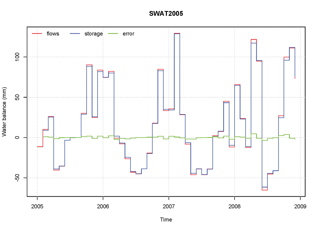
As it can be seen, the mass balance error (BAL) is one to two orders of magnitude smaller than the flows or the variation in storage. That’s pretty decent, I think.
Please, note that I only had SWAT2005 output files at hand, so the balance for the snowpack is only approximate (since sublimation is not taken into account) and also QTILE is missing. Also, LATQ_CNT is not reported on SWAT2005, so I used LATQ instead. On SWAT2012 output these terms are correctly outputted in output.hru, so the error should be lower. The absence of the lagged terms surf_bs and bss even in SWAT2012 may still generate a little mass balance error, but I could not test this since I only had SWAT2005 output.
The following plot shows the flows, storage variation and mass balance error as computed from a SWAT2005 output.hru file, for a number of years in one random HRU.

Sin comentarios